While designing/ working on my APRS project, I used LTSpice IV for some simulations. For those that don’t know, LTspice IV is a high performance SPICE simulator, schematic capture and waveform viewer from Linear Technology. It is a freeware and can be downloaded from this link. Versions for my both platforms exist, Win 7.0 and Mac. I like better the Win version. Is much more polished and has some features that are not available under Mac (e.g. schematic capture export as image).
I find SPICE simulations fascinating so I will probably start a series of posts on the topic. It is not a bullet proof method of testing a project, testing is much more reliable done in the old–fashioned way (hardware). But it is a very good method of guiding a project on the right track.
While adding the output filter I done some AC sweep analysis in LTSpice. AC sweep analyses in LTSpice can be used to analyze the frequency response of a circuit with fixed parameter values. If several parameter values need to be examined, you can either manually enter the values and simulate the circuit several times to view the response, or use the SPICE dot directive “.STEP”. The .STEP directive allows up to three parameters to be swept across an arbitrary range of values in a single simulation run. Consider the output filter from the APRS project:

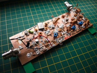
Prototype revision 3.0; this version includes a preamp to boost modulation and a simple modulation mechanism for the 144.0 MHz carrier. Note the output bandpass filter.
I created a new schematic in LTSpice just for the filter:

LTSPice IV 7-pole filter schematic. Standalone. Note the value and the label of the voltage source. Also note the way SPICE directives are added to the schematic. Each dot statement can be commented out using an asterisk.
Note that in above that the voltage source value has been changed to “AC 1” in preparation for an AC sweep to create a Bode plot, and the value of C10 and C9 has been changed to {C}, and for C5, C6, C7 and C11 to {Cp}; these allow the substitution of external values. The AC directive .ac dec 1k 50Meg 380Meg performs a logarithmic sweep from 50 MHz to 380 MHz, with 1,000 points per decade. This is practically useful, since it lets us view the range of possible corner frequency settings. Both .param directive inserts a temporary value for the capacitor of 18pF (for C10 — {C}) and 22pF (for C5, C6, C7 and C11 — {Cp}). Performing a simulation on the circuit above (Simulate Menu->Run or Alt-S-R) yields the Bode plot shown below:

Amplitude vs. frequency response for the 9-pole 2m output bandpass filter. Simulation done for an AC step response between 50 MHz and 380 MHz, 1,000 steps / octave — .ac oct 1k 50Meg 380Meg.
Note that the cutoff frequency appears to be around 136.7 MHz and 151.7 MHz, with a pass band of apx 15 MHz centred on 144 MHz. The frequency axis is shown on a logarithmic scale:
 two measurement cursors, click on the name of the plot (in this case is \"V(n008)\"). When inserting cursors, the values' pane is automatically displayed side-by-side with the graph. Note here the cutoff (-3 dB) frequencies and the filter bandwidth (\"Delta Frequency\") of apx 15 MHz.")
LTSpice IV: Zooming in a specific area of the graph is done by dragging a rectangle over the area of interest. To insert up to (max) two measurement cursors, click on the name of the plot (in this case is “V(n008)”). When inserting cursors, the values’ pane is automatically displayed side-by-side with the graph. Note here the cutoff (-3 dB) frequencies and the filter bandwidth (“Delta Frequency”) of apx 15 MHz.
The above simulation works well for simulating with a single component value (18pF and 22pF), but what if 3 or 5 capacitor values need to be tested ? One solution would be to change the .param directive that we set up earlier five times and run the simulation repeatedly to create five separate Bode plots. A more elegant solution is to use the SPICE dot directive .step to automatically insert the parameter values for us. For example, to test capacitors from 10pF to 22pF in 2pF steps, the directive .step param C 10pF 22pF 2pF could be used. This steps the parameter C through the requested value range in a linear fashion. The directive can be added to the circuit diagram and yields the Bode plot shown below:

LTSpice Parameter Sweep: .step param C 10pF 22pF 2pF yields the bode plot in the left pane. The right pane displays the zoomed peak area. Note the effect of sweeping values of {C} parameter: bandwidth stays roughly the same, however cutoff frequencies move to the left with the {C} parameter increasing in value. Light green — lowest value for {C}: 10pF; dark green — highest value for {C}: 22pF; purple is the default value of 18pF, as designed.
That’s for an introductory post on the parameter sweep in LTSpice. I find it extremely useful. Check out these interesting links too:
- Linear Technology web universe. One of the best among the best in electronics. Linear Technology Corporation has been designing, manufacturing and marketing a broad line of high performance analog integrated circuits for major companies worldwide for three decades.
- LTSpice IV pages. You might also wanna check LTPowerCAD (a complete power supply design tool program) and some SPICE models for amplifier simulation
- LTSpice Demo Circuits; These demo circuits are designed to ensure proper performance and have been reviewed by Linear Technology’s factory applications group. Follow the instructions to run the demo circuits in LTspice.